基于mit6.006的作业解析
hw1
时间复杂度分析
对这种形式的函数可以这样比较
\[f_1=n^{\sqrt{n}}=(2^{lgn})^{\sqrt{n}}\] \[f_2=n^{10}.2^{n/2}=2^{lg(10n)+n/2}\]
复杂度计算
对于T(n,n): T (x, y) = Θ(x + y) + T (x/2, y/2). 化成
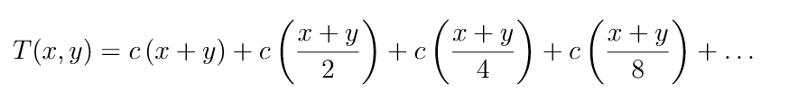
得到θ(n)
T (x, y) = Θ(x) + T (x, y/2). 等于lgy个θ(x) 即,θ(nlgn)
T (x, y) = Θ(x) + S(x, y/2), S(x, y) = Θ(y) + T (x/2, y).
化成T (x, y) = Θ(x) + Θ(y/2) + T (x/2, y/2). 与第一个例子相似,θ(n)
寻峰算法
1 | def algorithm1(problem, trace = None): |
算法一二如课程笔记所述,均是正确的,以下是证明
- algo1
- 证明算法不可能返回一个空值,首先算法不可能得到一个负索引的子数组(在只有一列的时候必然会得到结果而不是继续划分),在最小问题的情况下,如果此时子问题有一列,那么必然返回一个峰值,如果有两列,不管目前讨论的列是不是最大值,都会递归成最小为1为列的子问题,不会返回空值
- 证明返回的位置确实是峰值位置,如果算法1返回一个位置(r1,c1),则该位置必须具有列c1中的最大值,并且必须是某个递归子问题中的峰值。为了推导矛盾,假设(r1,c1)不是原始问题中的峰值。在某个子问题中,位置(r1,c1)与列c2相邻(|c1 - c2| = 1),并且值必须满足不等式val(r1,c1)< val(r1,c2)。
让(r2,c2)是算法1在c2列中找到的最大值的位置。因此,必定有val(r1,c2)≤ val(r2,c2)。因为c2是分割线,且算法选择在包含(r1,c1)的一半上进行递归,所以我们知道val(r2,c2)< val(r2,c1)。因此,我们有以下不等式链:
val(r1,c1)< val(r1,c2)≤ val(r2,c2)< val(r2,c1)
但是,为了使算法1将(r1,c1)作为峰值返回,(r1,c1)处的值必须是其列中的最大值,即val(r1,c1)≥ val(r2,c1)。因此,我们得到了一个矛盾。
- algo3是错误的
时间复杂度是θ(n),情况类似复杂度题目的第一个情况,1+1/2+1/4……
反例
如图所示的反例会选择返回一个在当前子问题中看起来像一个峰值,但是与子问题外部的某个更大值相邻的位置
| 0 | 0 | 9 | 8 | 0 | 0 | 0 |
|---|---|---|---|---|---|---|
| 0 | 0 | 0 | 0 | 0 | 0 | 0 |
| 0 | 1 | 0 | 0 | 0 | 0 | 0 |
| 0 | 2 | 0 | 0 | 0 | 0 | 0 |
| 0 | 0 | 0 | 0 | 0 | 0 | 0 |
| 0 | 0 | 0 | 0 | 0 | 0 | 0 |
| 0 | 0 | 0 | 0 | 0 | 0 | 0 |
| 0 | 0 | 0 | 0 | 0 | 0 | 0 |
对算法四的证明
- algo4
时间复杂度是θ(n),类似算法3
算法四交叉进行行和列的最大值寻找
- 如果峰值问题不为空,则算法将始终返回一个位置。在算法中,根据是在行还是列上分割,递归子问题的维度会相应地减少。所以算法要么在某个时刻停止并返回一个位置,要么最终检查一个行数或列数为非正的子问题。但是,问题的行数或列数变为严格负数的唯一方式是在某个时刻m=0或n=0。因此,如果算法没有返回位置,它必定最终检查一个空的子问题。然而,证明假设该情况不会发生。
- 如果算法返回一个位置,则该位置将是原始问题中的一个峰值。如果算法返回一个位置(r1, c1),那么该位置必定是某个递归子问题中的峰值。另外,如果(r2, c2)是算法执行过程中的最佳位置(存储在bestSeen变量中的位置),那么必定满足val(r1, c1) ≥ val(r2, c2)。证明假设(r1, c1)不是原始问题的峰值。那么当位置(r1, c1)通过递归调用链向上传递时,它必定在某个级别停止是不是峰值。因此,必定存在一个包含位置(r1, c1)的子问题,在该级别中,该子问题的某个邻居(r3, c3)的值满足val(r1, c1) < val(r3, c3)。对于(r3, c3)既是递归子问题的邻居又不包含在子问题中,它必定在算法的执行过程中被检查过。因此,必定满足val(r3, c3) ≤ val(r2, c2)。因此,我们得到以下不等式链:val(r1, c1) < val(r3, c3) ≤ val(r2, c2) ≤ val(r1, c1)。这导致了矛盾。
hw2
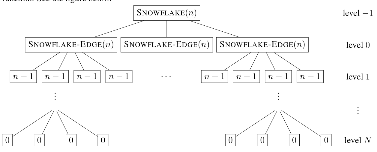
科赫雪花
1 | SNOWFLAKE(n) |
从主函数(层数视为-1)开始对每条边进行处理,这一层有三个节点。 而对边处理的函数则遵从这样的流程
- 把边等分成三个部分e1,e2,e3
- 对e1进行递归
- 以e2为一条边向外侧生成一个等边三角形,f2,g2是这个三角形的另外两条边
- 以此对f2,g2,e3进行递归 函数实际上把一条边拓展出了一个三角形 因此第i层的节点数是:\[3*4^i\]
3D 硬件加速渲染
在这种渲染方式中,cpu计算分解出的三角形顶点的集合,发给gpu进行绘制,因此cpu的执行时间只取决于分解出的三角形数量,也就是θ(4^n)
2D 硬件加速渲染
在这种渲染方式中,cpu实际上只计算不断分割出的线段集合,在本题中就是计算最外侧的轮廓的顶点的集合,计算结束后发给gpu绘制 时间复杂度依旧是θ(4^n),但需要注意的是由于计算完了才开始渲染,因此递归树的中间节点不会对渲染产生时间消耗
软件渲染
在没有硬件加速器的2D渲染(也称为软件渲染)中,CPU 像上一部分一样,为每个路径编译一个线段列表,但它也负责 用于“光栅化”每个线段。 光栅化获取线段端点的坐标 并计算位于线段上的所有像素的坐标。 用这些像素在显示器上绘制线段。光栅化算法在时间上的消耗与线段的长度成正比,线段上的像素数量与线段的长度成正比。 在整个问题中,假设所有线段的长度至少为一个像素,因此 光栅化的成本大于编译线段的成本。 需要注意的是:
- 中间节点依旧对渲染无影响
- 由于每次对边处理实际上增加了该边1/3的像素点,所以最后一层产生的代价是\[θ({(1/3)}^n)\]
- 同理,总渲染代价和cpu处理(只处理像素点)的时间复杂度都是\[θ({(4/3)}^n)\]
没有硬件加速的 3D 渲染
在这种情况下, CPU 编译三角形列表,然后光栅化每个三角形。 我们知道一种算法 栅格化一个三角形,其运行时间与三角形的表面积成正比。三角形内的像素数量与三角形的面积成正比。可以假设边长为 l 的三角形的面积为 θ(l^2)。 顺着递归树进行分析,首层只增加了三个节点,每个新节点对应一个边长是原边长1/3的新三角形,增加了1/3的面积,之后的每一层都有4^i个节点,对应4/9的面积增长,即每层的增长是 \[\frac{1}{3}.\frac{4}{9}^i\] 可以用等比数列的求和算出答案,但时间复杂度必然是θ(1)
电路模拟
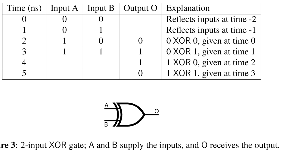 如图是对一个异或门的模拟,两个输入端AB产生的信号会在2ns的延迟后在输出端产生一个结果,除此以外没有延迟 按照题意运行
python -m cProfile -s time circuit.py < tests/5devadas13.in 得到如下结果(不完全),可以看到消耗最多时间的是lt(lower than)和find_min两个函数
1 | ncalls tottime percall cumtime percall filename:lineno(function) |
随后题意要求基于原来的api实现一个优先队列(最小堆)
1 | class PriorityQueue: |
python3可以运行所有测试,但无法运行可视化程序,不过也无所谓了,优化后再次运行一开始的输入
1 | ncalls tottime percall cumtime percall filename:lineno(function) |
问题解决了,amdtel的offer什么时候发?