实践报告
背景介绍
本次作业使用一个房价数据集,房价数据集完全由数字信息构成,规模属于中小级别(2w条左右),有一定的数据处理需求,但由于最主要的参数房价和其他相关列主要是简单的类线性关系,易于作为学习数据科学的入门材料。
问题描述
主要目标是预测房价,为此目标,需要清洗不合理的数据,寻找线性相关的列,最后利用一些回归模型来进行训练,并验证结果 最后的输入是数据集内和房价线性相关程度较高的列,输出则是对房价的预测结果。
数据描述
这些数据涉及在加州某个地区的街区以及基于 1990 年人口普查数据的一些汇总统计数据:
房屋中位价值:一个街区内家庭的房屋中位价值(以美元计算)
收入中位数:一栋房屋内的家庭收入中位数(以万美元衡量)
中位年龄:街区内房屋的中位年龄; 数字较小的是较新的建筑
房间总数:一个街区内的房间总数
卧室总数:一个街区内的卧室总数
人口:居住在一个街区内的总人数
家庭:一个街区的家庭总数
纬度:衡量房屋向北有多远的指标; 值越高越北 [°]
经度:衡量房屋向西有多远的量度; 数值越高,越西 [°]
距离海岸:到最近海岸点的距离[m]
到洛杉矶的距离:到洛杉矶市中心的距离[m]
到圣地亚哥的距离:到圣地亚哥中心的距离[m]
到圣何塞的距离: 到圣何塞中心的距离 [m]
到旧金山的距离:到旧金山市中心的距离[m]
Median House Value: Median house value for households within a block (measured in US Dollars)
Median Income: Median income for households within a block of houses (measured in tens of thousands of US Dollars)
Median Age: Median age of a house within a block; a lower number is a newer building [years]
Total Rooms: Total number of rooms within a block
Total Bedrooms: Total number of bedrooms within a block
Population: Total number of people residing within a block
Households: Total number of households, a group of people residing within a home unit, for a block
Latitude: A measure of how far north a house is; a higher value is farther north [°]
Longitude: A measure of how far west a house is; a higher value is farther west [°]
Distance to coast: Distance to the nearest coast point [m]
Distance to Los Angeles: Distance to the centre of Los Angeles [m]
Distance to San Diego: Distance to the centre of San Diego [m]
Distance to San Jose: Distance to the centre of San Jose [m]
Distance to San Francisco: Distance to the centre of San Francisco [m]
1 2 3 4 5 6 7 8 9 10 11 12 13 14 import numpy as npimport pandas as pd%matplotlib inline import matplotlib.pyplot as pltimport seaborn as snsimport warningswarnings.filterwarnings('ignore' ) np.random.seed(44 ) training_data = pd.read_csv('California_Houses.csv' )
1 training_data.columns.values
array(['Median_House_Value', 'Median_Income', 'Median_Age', 'Tot_Rooms',
       'Tot_Bedrooms', 'Population', 'Households', 'Latitude',
       'Longitude', 'Distance_to_coast', 'Distance_to_LA',
       'Distance_to_SanDiego', 'Distance_to_SanJose',
       'Distance_to_SanFrancisco'], dtype=object)
1 training_data.describe()
Median_House_Value
Median_Income
Median_Age
Tot_Rooms
Tot_Bedrooms
Population
Households
Latitude
Longitude
Distance_to_coast
Distance_to_LA
Distance_to_SanDiego
Distance_to_SanJose
Distance_to_SanFrancisco
count
20640.000000
20640.000000
20640.000000
20640.000000
20640.000000
20640.000000
20640.000000
20640.000000
20640.000000
20640.000000
2.064000e+04
2.064000e+04
20640.000000
20640.000000
mean
206855.816909
3.870671
28.639486
2635.763081
537.898014
1425.476744
499.539680
35.631861
-119.569704
40509.264883
2.694220e+05
3.981649e+05
349187.551219
386688.422291
std
115395.615874
1.899822
12.585558
2181.615252
421.247906
1132.462122
382.329753
2.135952
2.003532
49140.039160
2.477324e+05
2.894006e+05
217149.875026
250122.192316
min
14999.000000
0.499900
1.000000
2.000000
1.000000
3.000000
1.000000
32.540000
-124.350000
120.676447
4.205891e+02
4.849180e+02
569.448118
456.141313
25%
119600.000000
2.563400
18.000000
1447.750000
295.000000
787.000000
280.000000
33.930000
-121.800000
9079.756762
3.211125e+04
1.594264e+05
113119.928682
117395.477505
50%
179700.000000
3.534800
29.000000
2127.000000
435.000000
1166.000000
409.000000
34.260000
-118.490000
20522.019101
1.736675e+05
2.147398e+05
459758.877000
526546.661701
75%
264725.000000
4.743250
37.000000
3148.000000
647.000000
1725.000000
605.000000
37.710000
-118.010000
49830.414479
5.271562e+05
7.057954e+05
516946.490963
584552.007907
max
500001.000000
15.000100
52.000000
39320.000000
6445.000000
35682.000000
6082.000000
41.950000
-114.310000
333804.686371
1.018260e+06
1.196919e+06
836762.678210
903627.663298
数据处理
导入python库
封装函数
1 2 3 4 5 6 7 8 9 10 11 12 13 14 15 16 17 18 19 20 21 22 23 24 25 26 27 28 29 30 31 32 33 34 35 36 37 38 39 40 41 42 43 44 45 46 47 48 49 50 51 52 53 54 55 56 57 58 59 60 61 62 63 64 65 66 67 def remove_outliers (data, variable, lower=-np.inf, upper=np.inf ): df = data.copy() df = df[df[variable] > lower] df = df[df[variable] < upper] return df def train_val_split (data, train_pct=0.8 ): data_len = data.shape[0 ] shuffled_indices = np.random.permutation(data_len) split_index = int (0.8 * data_len) train_indices = shuffled_indices[:split_index] val_indices = shuffled_indices[split_index:] train = data.iloc[train_indices] validation = data.iloc[val_indices] return train, validation def plot_distribution (data, label ): fig, axs = plt.subplots(nrows=2 ) sns.histplot( data[label], ax=axs[0 ] ) sns.boxplot( x=data[label], ax=axs[1 ], showfliers=False ) spacer = np.max (data[label]) * 0.05 xmin = np.min (data[label]) - spacer xmax = np.max (data[label]) + spacer axs[0 ].set_xlim((xmin, xmax)) axs[1 ].set_xlim((xmin, xmax)) plt.subplots_adjust(hspace=0 ) fig.suptitle("Distribution of " + label) def draw_mean_lineplot (dis,val,df=training_data,thisbins=200 ): categories = pd.cut(df[dis], bins=thisbins) mids = [c.mid for c in categories] df['distance_bin' ] = mids mean_price = df.groupby('distance_bin' )[val].mean() newdf=pd.DataFrame() newdf['mean_price' ]=mean_price newdf['distance_bin' ]=mean_price.index sns.lineplot(x='distance_bin' ,y='mean_price' ,data=newdf) plt.title("mean house price with the same " +dis) plt.show() def draw_lmplot (x_col,name,y_col="Median_House_Value" ,bins=100 ,ci=1 ): sns.lmplot(data = training_data, x = x_col, \ y = y_col,x_bins=bins,x_ci=ci) plt.title("proportion of " +name+" against house value" ); def draw_jonitplot (x_col,name,y_col="Median_House_Value" ): sns.jointplot(data = training_data, x = x_col, \ y = y_col, \ kind = "hex" ) plt.suptitle(name+" agginst value" )
数据过滤
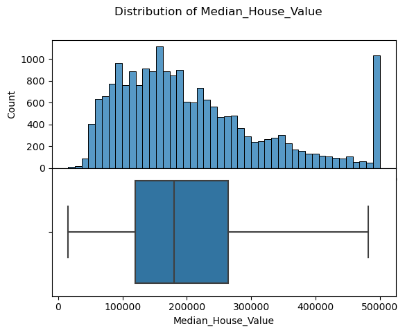
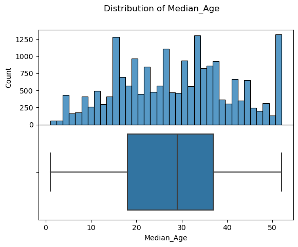
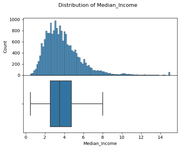
1 2 3 4 plot_distribution(training_data, label='Median_House_Value' ) plot_distribution(training_data, label='Median_Age' ); plot_distribution(training_data, label='Median_Income' );
png
png
png
可以看到收入和售价数据的右侧末端比较不合理,应该过滤
1 2 3 4 training_data=remove_outliers(training_data,'Median_Income' ,0 ,8 ) training_data=remove_outliers(training_data,'Median_House_Value' ,0 ,400000 ) training_data=remove_outliers(training_data,'Distance_to_coast' ,0 ,70000 ) training_data=remove_outliers(training_data,'Households' ,0 ,1500 )
1 training_data.describe()
Median_House_Value
Median_Income
Median_Age
Tot_Rooms
Tot_Bedrooms
Population
Households
Latitude
Longitude
Distance_to_coast
Distance_to_LA
Distance_to_SanDiego
Distance_to_SanJose
Distance_to_SanFrancisco
count
14651.000000
14651.000000
14651.000000
14651.000000
14651.000000
14651.000000
14651.000000
14651.000000
14651.000000
14651.000000
1.465100e+04
1.465100e+04
14651.000000
14651.000000
mean
199561.517917
3.696580
29.953996
2356.678657
496.034742
1367.255341
468.929561
35.372597
-119.555017
21259.751408
2.490542e+05
3.721187e+05
359123.874456
397236.235539
std
79310.711796
1.419884
12.191439
1425.953928
287.919292
814.994880
266.065608
2.077014
2.063217
16562.862059
2.475190e+05
2.905277e+05
226985.441402
262135.238533
min
14999.000000
0.499900
1.000000
11.000000
3.000000
3.000000
3.000000
32.540000
-124.350000
120.676447
4.205891e+02
4.849180e+02
569.448118
456.141313
25%
140600.000000
2.625000
20.000000
1410.000000
296.000000
816.000000
286.000000
33.880000
-121.890000
8077.199272
2.631262e+04
1.550810e+05
88700.495102
92070.783507
50%
187500.000000
3.551100
31.000000
2053.000000
431.000000
1190.000000
412.000000
34.140000
-118.360000
17596.867293
1.385490e+05
1.872540e+05
484362.783196
552023.712780
75%
252000.000000
4.625000
38.000000
2968.000000
631.000000
1725.000000
595.000000
37.690000
-117.980000
28063.195081
5.221622e+05
7.009827e+05
519935.107297
587792.558476
max
399400.000000
7.988700
52.000000
12837.000000
2219.000000
8733.000000
1499.000000
41.950000
-114.550000
69995.382339
1.018260e+06
1.196919e+06
836762.678210
903627.663298
数据分析——寻找与房屋价格有线性关系的列
可视化房屋价格与距离远近的关系
1 2 3 places=['Distance_to_coast' , 'Distance_to_LA' , 'Distance_to_SanDiego' , 'Distance_to_SanJose' , 'Distance_to_SanFrancisco' ]
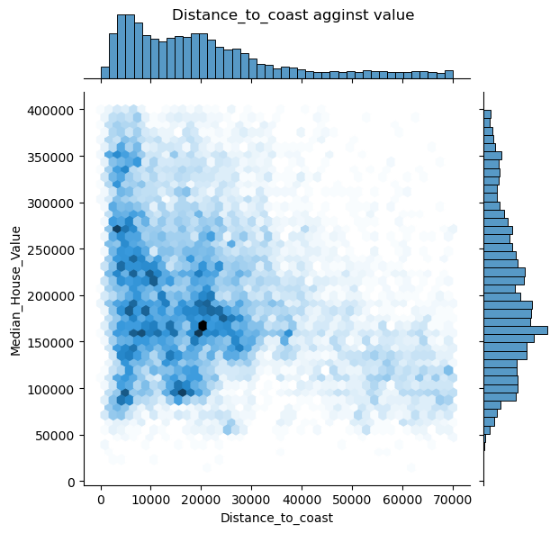
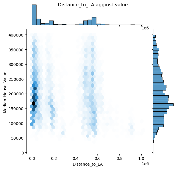
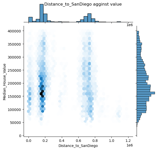
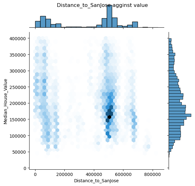
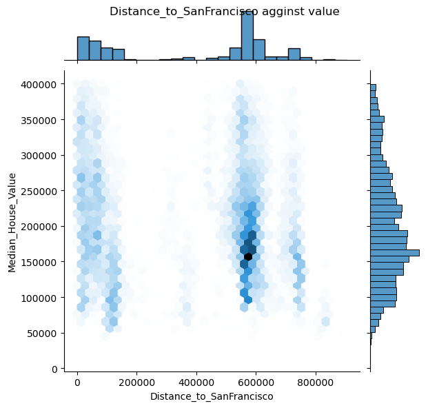
1
2
for pla in places: draw_jonitplot(x_col=pla,name=pla)
png
png
png
png
png
可以看出其中只有距海岸线距离似乎与房价有关系
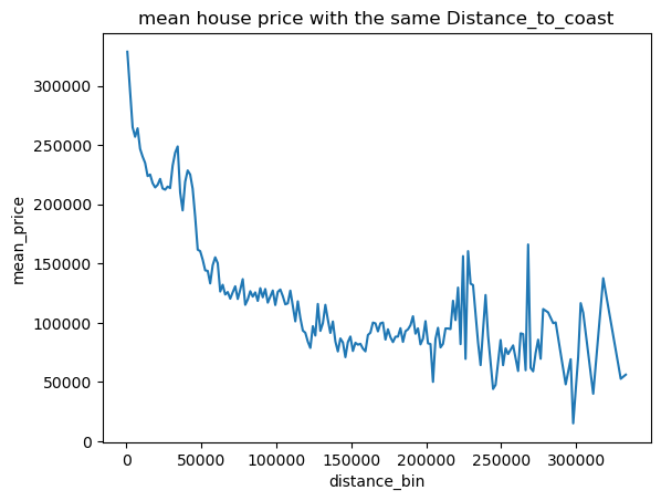
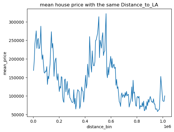
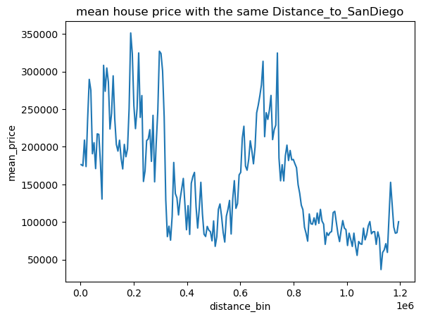
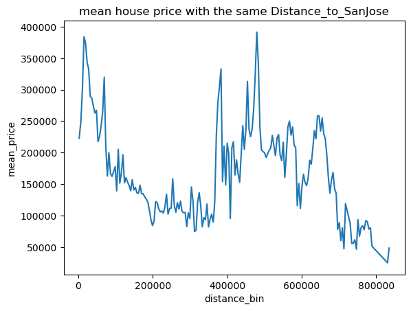
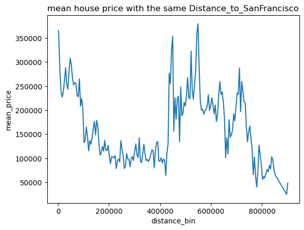
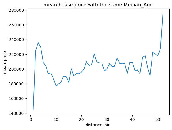
用更直观的折线图表示平均房价与海岸线与城市距离关系
1
2
for pla in places: draw_mean_lineplot(dis=pla,val='Median_House_Value' )
png
png
png
png
png
根据可视化发现,只有海岸线距离与房价有类似线性关系
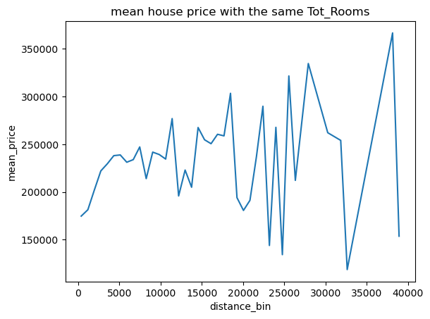
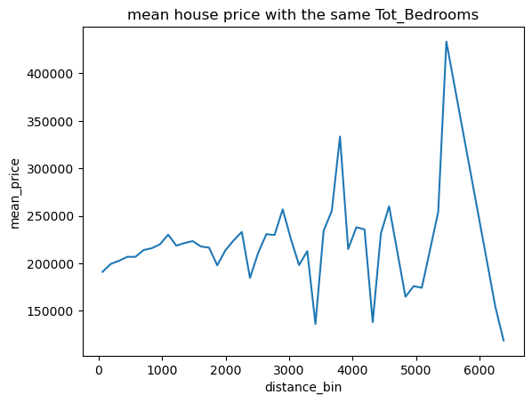
房屋数和卧室数与房价是否相关
1 2 draw_mean_lineplot(dis='Tot_Rooms' ,val='Median_House_Value' ,thisbins=50 ) draw_mean_lineplot(dis='Tot_Bedrooms' ,val='Median_House_Value' ,thisbins=50 )
png
png
可以看出单独两列和房价都无明显关系
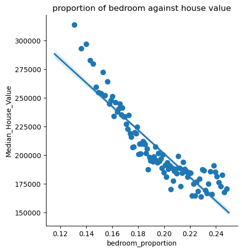
1 2 3 training_data['bedroom_proportion' ] =training_data['Tot_Bedrooms' ] / training_data['Tot_Rooms' ] training_data=remove_outliers(training_data,'bedroom_proportion' ,0 ,0.25 ) draw_lmplot(x_col='bedroom_proportion' ,name='bedroom' )
png
两者比例和房价近似线性有关
和房屋年龄关系
1 draw_mean_lineplot(dis='Median_Age' ,val='Median_House_Value' ,thisbins=500 )
png
可以看出和年龄没有明显关系
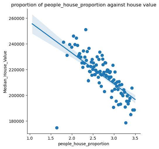
和家庭平均人口数的关系
1 2 3 training_data['people_house_proportion' ] =training_data['Population' ] / training_data['Households' ] training_data=remove_outliers(training_data,'people_house_proportion' ,0 ,3.5 ) draw_lmplot(x_col='people_house_proportion' ,name='people_house_proportion' )
png
1 training_data['people_house_proportion' ].describe()
count    9213.000000
mean        2.722022
std         0.422372
min         1.060606
25%         2.432647
50%         2.740845
75%         3.044444
max         3.499266
Name: people_house_proportion, dtype: float64
可以看出和家庭平均人数有近似线性关系
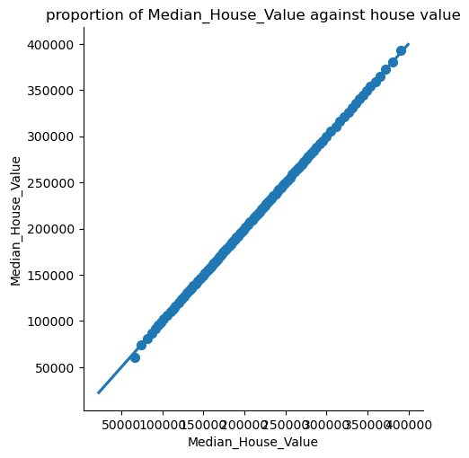
与中位数收入的关系
1 draw_lmplot(x_col='Median_House_Value' ,name='Median_House_Value' ,ci=95 )
png
可以看出和中位数收入线性有关
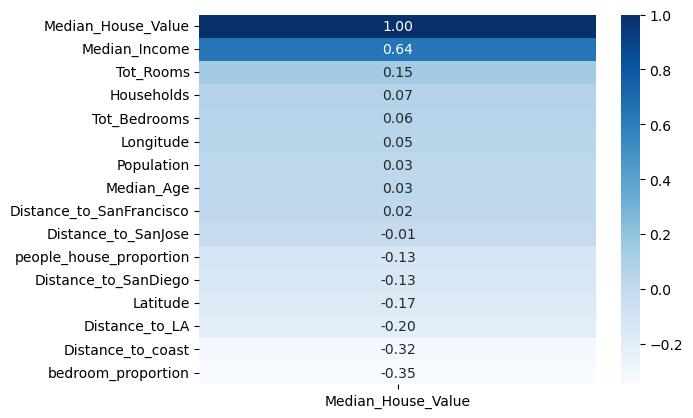
验证——相关性可视化
1
2
3
correlation = training_data.corr()['Median_House_Value' ].sort_values(ascending = False ).to_frame() sns.heatmap(correlation, annot = True , cmap = 'Blues' , fmt = '.2f' )
<Axes: >
png
建立模型
由于数据呈现出较为标准的线性关系,选取了线性回归,决策树,随机森林,k近邻回归等回归模型,这些模型适合处理线性数据关系,并且其原理和训练方法容易理解。 缺点则是都是比较简单的模型,因此准确度不算特别理想,也不适宜处理关系复杂的数据
1 2 3 4 5 6 7 8 9 10 11 12 13 14 15 16 17 18 19 20 21 22 23 def divide_datas (train,valid,list ): X_train = train[list ] y_train = train[['Median_House_Value' ]] X_valid = valid[list ] y_valid = valid[['Median_House_Value' ]] return X_train,y_train,X_valid,y_valid def series_to_df (predict ): predictions_series = pd.Series(predict[:,0 ]) predictions_df = predictions_series.to_frame() predictions_df=predictions_df.rename(columns={0 : 'house_value' }) return predictions_df def to_series (predict ): s = pd.Series(predict) df = s.to_frame() return df.values
1
2
3
4
5
6
7
train_m1, valid_m1 = train_val_split(training_data) train_m2, valid_m2 = train_val_split(training_data) features=['Median_Income' ,'Distance_to_coast' ,'bedroom_proportion' ,'people_house_proportion' ] X_train_m1,y_train_m1,X_valid_m1,y_valid_m1 = divide_datas(train_m1,valid_m1,['Median_Income' ]) X_train_m2,y_train_m2,X_valid_m2,y_valid_m2 = divide_datas(train_m2,valid_m2,features)
建立线性模型
\[
\hat{y}_i = \theta_0 + \theta_1 x_i
\]
建立线性回归模型,并可视化预测值的分布与实际分布比较
1
2
3
4
5
6
7
8
9
from sklearn import linear_model as lmlinear_model_m1 = lm.LinearRegression() linear_model_m2 = lm.LinearRegression() linear_model_m1.fit(X_train_m1, y_train_m1) y_predicted_m1 = linear_model_m1.predict(X_valid_m1) predictions_df=series_to_df(y_predicted_m1)
1
2
3
linear_model_m2.fit(X_train_m2, y_train_m2) y_fitted_m2 = linear_model_m2.predict(X_train_m2) y_predicted_m2 = linear_model_m2.predict(X_valid_m2)
1 linear_model_m1.score(X_train_m1, y_train_m1)
0.4054567472597721 linear_model_m2.score(X_train_m2, y_train_m2)
0.5238399282191235可以看出使用更多特征列的模型二有更好的性能
主成分分析(PCA)
1
2
3
4
5
6
7
8
9
10
11
12
13
14
15
16
17
18
from sklearn.decomposition import PCAlinear_model_m3 = lm.LinearRegression() train_m3, valid_m3 = train_val_split(training_data) X_train_m3,y_train_m3,X_valid_m3,y_valid_m3 = divide_datas(train_m3,valid_m3,features) pca = PCA(n_components=4 ) pca.fit(X_train_m3) principal_components = pca.transform(X_train_m3) pca.fit(X_valid_m3) principal_components_valid = pca.transform(X_valid_m3) linear_model_m3.fit(principal_components, y_train_m3) y_fitted_m3 = linear_model_m3.predict(principal_components) y_predicted_m3 = linear_model_m3.predict(principal_components_valid)
1
2
linear_model_m3.score(principal_components, y_train_m3)
0.5185359815322779正则化
1 2 3 4 5 lasso_model = lm.Lasso(alpha=3 ) lasso_model.fit(X_train_m3, y_train_m3) y_predicted_lasso = lasso_model.predict(X_valid_m3) y_predicted_lasso=to_series(y_predicted_lasso)
1 2 3 4 ridge_model = lm.Ridge(alpha=3 ) ridge_model.fit(X_train_m3, y_train_m3) y_predicted_ridge = ridge_model.predict(X_valid_m3)
1 ridge_model.score(X_train_m3, y_train_m3)
0.51771357592197531 lasso_model.score(X_train_m3, y_train_m3)
0.5185322538476318决策树模型
1 2 3 4 5 6 from sklearn import treedecision_tree_model = tree.DecisionTreeClassifier(max_depth=50 ,min_samples_split=4 ) decision_tree_model = decision_tree_model.fit(X_train_m3, y_train_m3) y_predicted_tree=decision_tree_model.predict(X_valid_m3) y_predicted_tree=to_series(y_predicted_tree)
1 2 3 4 5 decision_tree_model_regression = tree.DecisionTreeRegressor(criterion='absolute_error' ,min_samples_split=3 ) decision_tree_model_regression = decision_tree_model_regression.fit(X_train_m3, y_train_m3) y_predicted_tree_regression=decision_tree_model_regression.predict(X_valid_m3) y_predicted_tree_regression=to_series(y_predicted_tree_regression)
1 decision_tree_model.get_depth()
501 2 3 4 5 from sklearn.ensemble import RandomForestRegressorforest_model = RandomForestRegressor(criterion='absolute_error' ,max_depth=50 ,random_state=0 ,min_samples_leaf=3 ,n_jobs=4 ) forest_model = forest_model.fit(principal_components,y_train_m3)
1 2 y_predicted_forest=forest_model.predict(principal_components_valid) y_predicted_forest=to_series(y_predicted_forest)
k近邻回归
1 2 3 4 from sklearn.neighbors import KNeighborsRegressorKE_model=KNeighborsRegressor(n_neighbors=2 ,weights='distance' ) KE_model=KE_model.fit(X_train_m3,y_train_m3) y_predicted_ke=KE_model.predict(X_valid_m3)
模型评估
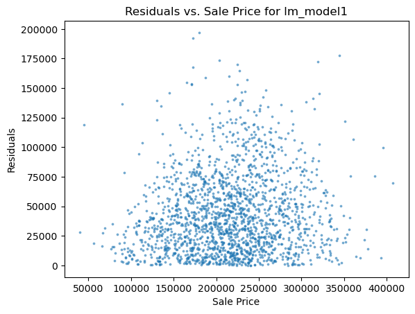
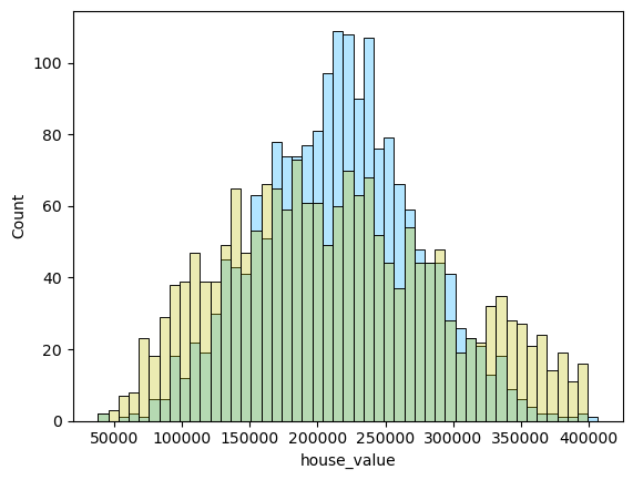
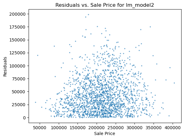
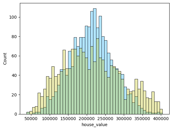
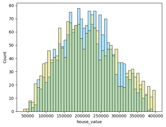
1 2 3 4 5 6 7 8 9 10 11 12 13 14 15 16 17 18 19 20 21 22 23 24 25 26 27 28 29 30 31 32 33 34 35 36 37 38 39 40 41 42 def rmse (predicted, actual ): return np.sqrt(np.mean((actual - predicted)**2 )) def mae (predicted,actual ): return np.mean(np.abs (predicted - actual)) def accuracy (preditcted,actual,num=500 ): return (abs (preditcted - actual)<=num).mean().mean() def evaluate_model (predicted,valid,num=500 ): rmse_val = rmse(predicted, valid) mae_val = mae(predicted,valid) accuracy_val = accuracy(predicted,valid,num) return {'rmse' : rmse_val, 'mae' : mae_val, 'accuracy' : accuracy_val} def make_result (predicts,df ): for predict in predicts: df.loc[len (df)] = evaluate_model(predict, y_valid_m3,10000 ) return df def scatter_plot (predict,actual,name ): residuals = abs (predict - actual) plt.scatter(predict, residuals, alpha=0.5 , s=3 ) plt.xlabel('Sale Price' ) plt.ylabel('Residuals' ) plt.title('Residuals vs. Sale Price for ' +name) ax=axs[1 ] plt.show() def two_x_histplot (df1,df2,col1,col2 ): min_value = min (df1[col1].min (), df2[col2].min ()) max_value = max (df1[col1].max (), df2[col2].max ()) bins = np.linspace(min_value, max_value, 50 ) sns.histplot(data=df1, x=col1, alpha=0.5 ,bins=bins,color='#66ccff' ) sns.histplot(data=df2, x=col2, alpha=0.3 ,bins=bins,color='y' ) ax=axs[0 ] plt.show()
1 2 3 4 5 6 7 8 results = pd.DataFrame(columns=['rmse' , 'mae' , 'accuracy' ]) results.loc[len (results)] = evaluate_model(y_predicted_m1, y_valid_m1,10000 ) results.loc[len (results)] = evaluate_model(y_predicted_m2, y_valid_m2,10000 ) pres=[y_predicted_m3,y_predicted_lasso,y_predicted_ridge,y_predicted_tree,y_predicted_tree_regression,y_predicted_forest,y_predicted_ke] results=make_result(pres,results) results.index=['lm_model1' ,'lm_model2' ,'lm_pca_model3' ,'lasso' ,'ridge' ,'tree' ,'tree_regression' ,'forest_regression' ,'K_neighbours' ] results
rmse
mae
accuracy
lm_model1
60922.482902
48571.055228
0.135648
lm_model2
56846.626574
43979.354330
0.160608
lm_pca_model3
55342.558354
43704.366177
0.154097
lasso
55311.818220
43551.728305
0.150841
ridge
55434.380284
43656.940158
0.150841
tree
77547.042415
58941.074335
0.141617
tree_regression
73484.094196
56195.496473
0.127509
forest_regression
52955.981209
40886.882257
0.170917
K_neighbours
74706.010594
52427.281809
0.204558
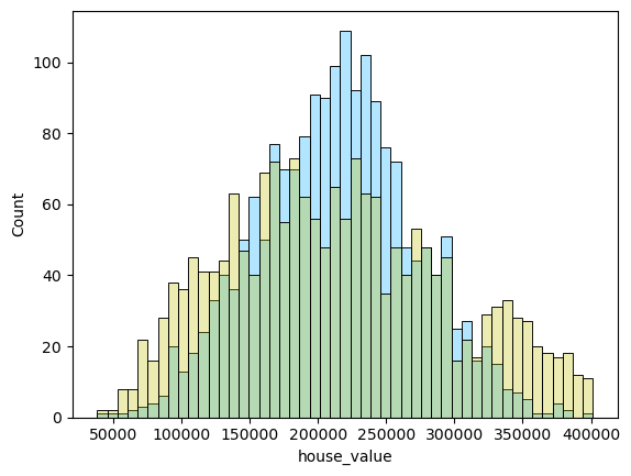
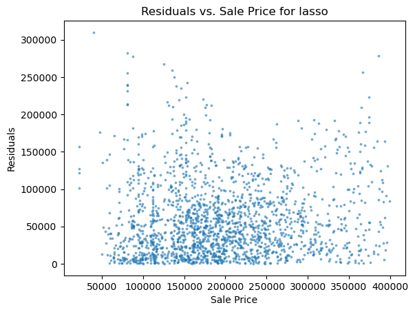
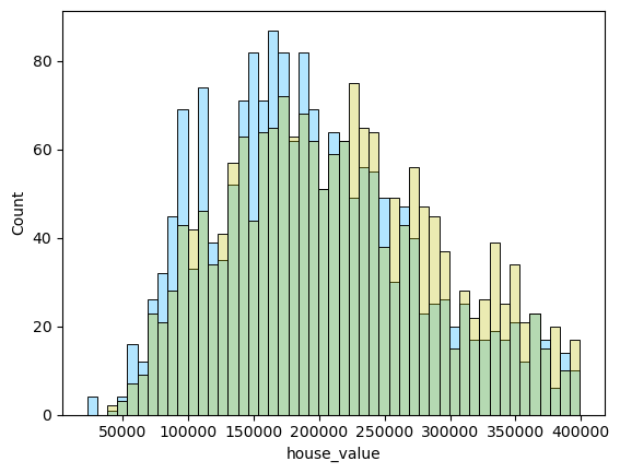
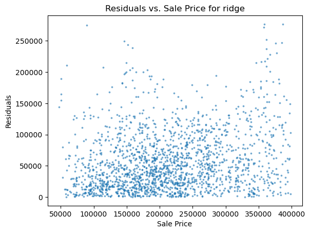
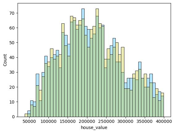
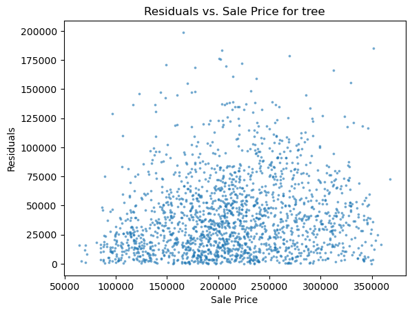
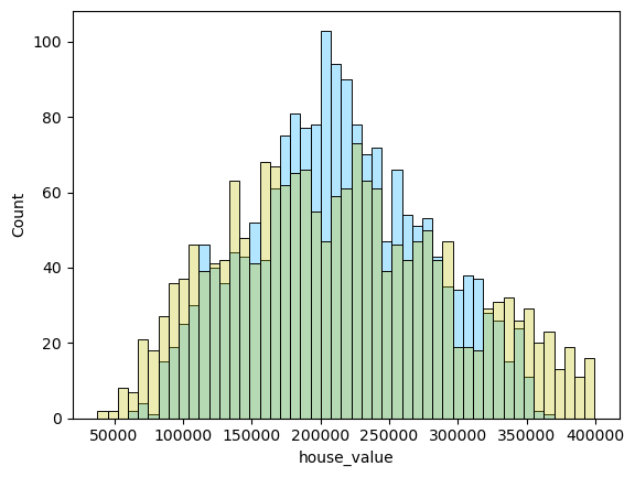
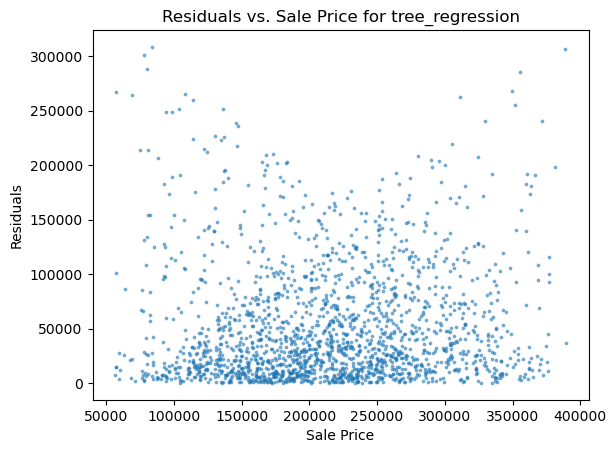
1 2 3 4 5 6 for i in range (len (pres)): names=['lm_model1' ,'lm_model2' ,'lm_pca_model3' ,'lasso' ,'ridge' ,'tree' ,'tree_regression' ,'forest_regression' ,'K_neighbours' ] scatter_plot(pres[i],y_valid_m3,names[i]) two_x_histplot(series_to_df(pres[i]),y_valid_m3,"house_value" ,"Median_House_Value" ) plt.show()
png
png
png
png
png
png
png
png
png
png
png
png
png
png
交叉验证
1 2 3 4 5 6 7 8 9 from sklearn.model_selection import cross_val_predictdef cross_validation (mls,is_series ): result_df=pd.DataFrame(columns=['rmse' , 'mae' , 'accuracy' ]) for i in range (len (models)): predicted=cross_val_predict(mls[i], X_train_m3, y_train_m3, cv=10 ,n_jobs=-1 ) if (is_series[i]): predicted=to_series(predicted) result_df.loc[len (result_df)]=evaluate_model(predicted, y_train_m3,10000 ) return result_df
1
2
3
4
5
linear_model_m1 = lm.LinearRegression() models=[linear_model_m3,lasso_model,ridge_model,decision_tree_model,decision_tree_model_regression,forest_model,KE_model] tf=[0 ,1 ,0 ,1 ,1 ,1 ,0 ] cross_results=cross_validation(models,tf) cross_results.index=['lm_model' ,'lasso' ,'ridge' ,'tree' ,'tree_regression' ,'forest_regression' ,'K_neighbours' ]
rmse
mae
accuracy
lm_model
55984.041030
43744.485025
0.150611
lasso
55984.270526
43748.196798
0.151018
ridge
56032.724551
43836.923361
0.149661
tree
76236.606876
58051.316147
0.139620
tree_regression
75482.497313
56896.289009
0.147083
forest_regression
53620.108361
40894.203324
0.174763
K_neighbours
76776.253905
55102.977787
0.192130